Pixel simulator
Pixel is an alternative PDE solver which uses the simple FTCS method to solve the PDE using the pixels of the geometry image as the grid.
Simulation options
The default settings should work well in most cases, but if desired they can be adjusted by going to Advanced->Simulation options
The simulation options that can be used to fine tune-the Pixel solver.
- Integrator
the explicit Runge-Kutta integration scheme used for time integration
default: 2nd order Heun scheme, with embedded 1st order error estimate
a higher order scheme may be more efficient if the maximum allowed error is very small
see the Time integration section for more information on the integrators
- Max relative local error
the maximum relative error allowed on the concentration of any species at any pixel
default: 0.005
local means the estimated error for a single timestep, at a single point
relative means each error estimate is divided by the species concentration
making this number smaller makes the simulation more accurate, but slower
- Max absolute local error
the maximum error allowed on the concentration of any species at any pixel
default: infinite
local means the estimated error for a single timestep, at a single point
absolute means the error estimate is not normalised by the species concentration
making this number smaller makes the simulation more accurate, but slower
- Max timestep
the maximum allowed timestep
default: infinite
- Multithreading
if enabled, multiple CPU threads can be used
default: disabled
enabling this can make simulations of large models run faster
however it can also make small models run slower
- Max CPU threads
limit the maximum number of CPU threads to be used
default: unlimited
- Symbolic optimization
factor out common subexpressions when constructing the reaction terms
default: enabled
- Compiler optimization level
how much optimization is done when compiling the reaction terms
default: 3
Spatial discretization
Space is discretized using a linear grid with spacing \(\delta x\), \(\delta y\), \(\delta z\). The concentration is defined as a 3d array of values \(c_{i,j,k}\), where the value with index \((i,j,k)\) corresponds to the concentration at the voxel-centre spatial point \((x = x_0 + (i+\frac{1}{2}) \delta x, y = y_0 + (j+\frac{1}{2}) \delta y, z = z_0 + (k+\frac{1}{2}) \delta z)\), where \((x_0,y_0,z_0)\) is the model geometry origin.
For spatially varying self-diffusion constants, the diffusion term is written in conservative form. With species storage coefficient \(S \geq 0\), the PDE for one species is
and discretized using face fluxes with arithmetic averaging of \(D\) at neighbouring voxels. For one species in voxel \((i,j,k)\):
with face diffusion constants
and similarly in \(y,z\) (and for the minus faces).
This has \(\mathcal{O}(\delta x^2)+\mathcal{O}(\delta y^2)+\mathcal{O}(\delta z^2)\) discretisation errors. Inserting this approximation into the reaction-diffusion equation converts the PDE into a system of coupled ODEs.
If \(D\) is spatially constant, this reduces to the usual central-difference Laplacian form.
Cross-diffusion
If cross-diffusion is enabled, Pixel solves for each target species \(s\)
where \(D_{s,r}\) is the cross-diffusion coefficient that maps gradients of species \(r\) to flux of species \(s\). The same conservative face-flux stencil is applied term-by-term: for each pair \((s,r)\), Pixel adds a face-averaged discretization of \(\nabla \cdot (D_{s,r}\nabla c_r)\) to species \(s\).
Space-dependent expressions
For spatially dependent reactions and cross-diffusion expressions, Pixel provides all three spatial coordinates as local variables per voxel: \(x\), \(y\), \(z\). These coordinates are the physical voxel-centre coordinates (including the geometry origin). The internal state vector therefore includes three spatial padding values (plus optional time), and these values are held constant during time integration.
Step-by-step derivation
For one species (without cross-diffusion), start from
Integrate over one voxel \(V_{i,j,k}\)
Assumptions:
\(D(\mathbf{x})\) is isotropic (scalar), but may vary in space
\(R\) is local in space (depends on the state at the same point)
Apply the divergence theorem to the diffusion term
This is the sum of six face flux integrals (\(x^\pm, y^\pm, z^\pm\)).
Replace volume/face integrals by midpoint (cell-centered) approximations
Assumption: uniform Cartesian grid with voxel spacings \(\delta x,\delta y,\delta z\).
Define cell-center values \(c_{i,j,k}\approx c(\mathbf{x}_{i,j,k})\) and \(D_{i,j,k}\approx D(\mathbf{x}_{i,j,k})\). Then
and similarly for the other faces.
Discretize face-normal gradients by central differences
and similarly for the minus face and for \(y,z\).
Approximate face diffusion constants from neighbouring cell values
Assumption: face diffusion is approximated by arithmetic interpolation of neighbouring voxel values:
(and similarly for \(y,z\)).
Assemble the semi-discrete ODE (method of lines)
Substituting the face fluxes into the surface-balance form and dividing by \(\delta x\,\delta y\,\delta z\) gives
where \(R_{i,j,k}\) is the cell-centered reaction term.
Local truncation error
Assumption: \(c\) and \(D\) are sufficiently smooth. Each directional term is second-order accurate on the uniform grid, so the spatial error is \(\mathcal{O}(\delta x^2)+\mathcal{O}(\delta y^2)+\mathcal{O}(\delta z^2)\).
Boundary handling
Assumption: zero-flux Neumann boundaries. Implementation-wise, an out-of-domain neighbour index is replaced by the boundary voxel itself, which makes the corresponding face gradient (and therefore face flux) zero.
Time integration
Time integration is performed using explicit Runge-Kutta integrators. Compared to implicit integrators, they are easier to implement and offer better performance (for the same timestep). However they become unstable if the timestep \(h\) is made too large, so in practice they can end up being slower than implicit methods for stiff problems, where the timestep is forced to be very small to maintain stability.
Integrators differ in their:
order of truncation error
order of embedded error estimate (if any)
number of stages (i.e. cost of a step)
region of stability (can be increased by adding more stages)
memory requirements
Implemented integrators:
- Euler
1st order solution
no error estimate
1 stage
- Embedded Heun / modified Euler
2nd order solution
1st order error estimate
2 stages
see e.g. eq (2.15) of https://doi.org/10.1016/0021-9991(88)90177-5
- Embedded Shu-Osher
3rd order solution
2nd order error estimate
3 stages
see eq (2.17) of https://doi.org/10.1016/0021-9991(88)90177-5
- RK4(3)5[3S*]
4th order solution
3rd order error estimate
5 stages
see alg.6 & tab.6 of https://doi.org/10.1016/j.jcp.2009.11.006
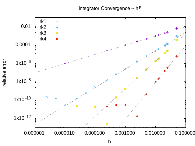
An example of the convergence of the included RK integrators: relative error of the solution at a particular pixel as a function of the stepsize.
These integrators have three sources of error:
- Round-off error due to finite precision
mostly only relevant for high order solvers: not relevant here
- Truncation error due to finite order of integration scheme
we are generally forced by the diffusion term to make the timestep small to maintain stability
also no benefit from making the time integration errors significantly smaller than the spatial discretisation errors
so this is also typically not a concern
- Numerical instability of integrator
a problem when ODEs become stiff, e.g. high rate of diffusion, stiff reaction terms
avoiding these instabilities is our main concern
Adaptive timestep
We use the embedded lower order solution to estimate the error at each timestep, and use this to adapt the stepsize during the integration:
RK gives us a pair of \(u_{n+1}^{(p)} = u_{n} + \mathcal{O}(h^{p+1})\) solutions
difference between \(p, p-1\) solutions gives local error of order \(\mathcal{O}(p)\)
to get the relative error we divide this by \(c = ( |c_{n+1}| + |c_{n}| + \epsilon)/2\)
we use the average of the old and new concentration, plus a small constant, to avoid dividing by zero
we do this for all species, compartments and spatial points, and take the maximum value
if this error is larger than the desired value, the whole step is discarded
the new timestep is given by \(0.98 dt_{old} (err_{desired}/err_{measured})^{1/p}\)
the 0.98 factor is slightly less than 1 to account for the higher order terms that are neglected here
it is better to have a slightly smaller timestep than to have to repeat the whole step
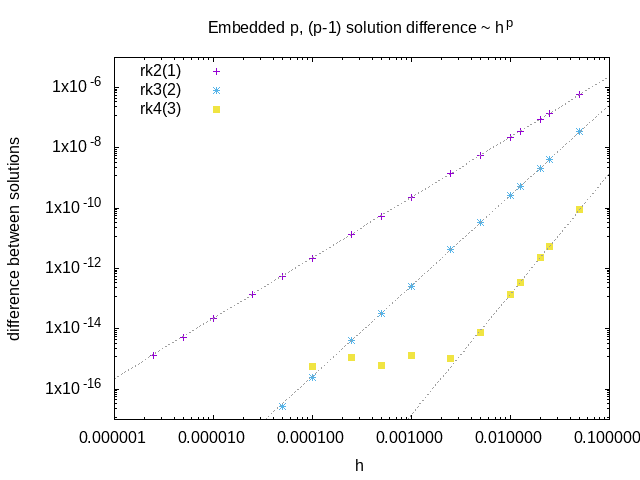
An example of the difference between order p and order p-1 solutions from embedded schemes as a function of the stepsize. This quantity is a measure of the local integration error, and scales like \(h^p\)
Maximum timestep
For the Euler method, we don’t have an embedded lower order solution from which we can estimate of the error, so we can’t automatically adjust the stepsize. However, if we ignore the reaction terms, there is an analytic upper bound on the size of timestep that can be used for Euler (see p125 of https://doi.org/10.1017/CBO9780511781438 ), above which the system becomes unstable:
where \(D_{\max}\) is an effective diffusion scale for the species, and \(S\) is that species’ storage coefficient.
Without cross-diffusion, \(D_{\max}\) is the largest self-diffusion value over all voxels. With cross-diffusion, Pixel uses a conservative bound based on
and applies the same CFL expression with \(D_{\max} = D_{\mathrm{eff},s}\).
So if the user selects a timestep larger than this, the simulator automatically reduces it to the above value to avoid the system becoming unstable. Note that the system can still become unstable if the reaction terms are stiffer than the diffusion terms.
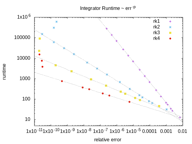
An example of the runtime of the RK integrators as a function of the relative error on the final solution. The higher order integrators offer better performance if a very accurate solution is required, but at lower accuracy the lower order integrators are much faster.
Boundary Conditions
The boundary condition for all boundaries is the “zero-flux” Neumann boundary condition. This is implemented in the spatial discretization by setting the concentration in the neighbouring pixel that lies outside the compartment boundary to be equal to the concentration in the boundary pixel value, or equivalently by setting the neighbour of each boundary pixel to itself.
Compartments
Each compartment is discretized, with the above boundary conditions applied for the diffusion term.
Membranes
Reactions that take place between two compartments involve a flux across the membrane separating the two compartments. For each neighbouring pair of pixels from the two compartments, whose common boundary constitutes the membrane, the flux term is converted into a reaction term that creates or destroys the appropriate amount of species concentration in each pixel.
Zero-storage species
When a species has storage coefficient \(S = 0\), its PDE becomes an algebraic constraint:
If cross-diffusion terms are present, the same generalized diffusion operator from the
Cross-diffusion section is used in this constraint.
Rather than being integrated forward in time, the concentration of such a species must satisfy this constraint at every timestep. The Pixel solver handles this via operator splitting with adaptive pseudo-time relaxation.
Operator splitting. Zero-storage species are excluded from the main Runge-Kutta time integration.
Their dcdt is set to zero by the storage term (since \(1/S\) is treated as zero),
so the RK stepper leaves their concentrations unchanged.
Instead, a separate constraint solver is called before each evaluation of the right-hand side
(i.e. before each RK stage), ensuring that time-integrated species always see
zero-storage concentrations that satisfy the constraint.
Adaptive pseudo-time relaxation. The constraint is solved by introducing a fictitious time \(\tau\) and integrating the pseudo-time equation
to steady state. This is done using the same embedded RK2(1)2 (Heun) integrator used for the main time integration, with adaptive step size control. The pseudo-timestep is bounded by the CFL stability condition:
where \(D_{\max}\) is the largest diffusion constant over all voxels for the zero-storage species.
Convergence criteria. The relaxation iterations stop when the residual \(r = \nabla \cdot (D \nabla c) + R\) is small enough. The same error tolerances (max absolute and max relative local error) configured for the main time integrator are used as convergence thresholds: the absolute residual must be below the configured max absolute error, and the relative residual (normalised by the species concentration) must be below the configured max relative error. A maximum of 100 iterations is allowed; if convergence is not reached, a warning is logged.
Error estimation. Zero-storage species are excluded from the main RK error estimation, since they are not time-integrated and their accuracy is controlled by the constraint solver instead.
CFL bound. Zero-storage species do not contribute to the maximum stable timestep for the main RK integrator, since the storage coefficient \(S\) appears in the numerator of the CFL bound (see the Maximum timestep section).
Special case: D = 0 and S = 0. When both diffusion and storage are zero, the constraint reduces to \(0 = R(c)\), a purely algebraic equation. The relaxation solver uses a fallback pseudo-timestep in this case, but convergence depends on the structure of \(R\).
Non-spatial species
A species can be ‘non-spatial’, which means that at each timestep, its time derivative is calculated as normal at each point in the compartment, but is then spatially averaged over the whole compartment. This can be used to approximate a species with a very high diffusion constant without requiring a correspondingly tiny timestep to maintain the stability of the solver.
Non-negativity clamp
After each accepted timestep, Pixel clamps negative primary-species concentrations to zero. This keeps concentrations physically meaningful and matches the behaviour of dune-copasi.