Getting started
Install and import sme
[1]:
!pip install -q sme
import sme
from matplotlib import pyplot as plt
import numpy as np

print("sme version:", sme.__version__)
Matplotlib is building the font cache; this may take a moment.
sme version: 1.12.0+103fb01
Importing a model
to load an existing sme or xml file:
sme.open_file('model_filename.xml')to load a built-in example model:
sme.open_example_model()
[2]:
my_model = sme.open_example_model()
Getting help
to see the type of an object:
type(object)to print a one line description of an object:
repr(object)to print a multi-line description of an object:
print(object)to get help on an object, its methods and properties:
help(object)
[3]:
type(my_model)
[3]:
sme.Model
[4]:
repr(my_model)
[4]:
"<sme.Model named 'Very Simple Model'>"
[5]:
print(my_model)
<sme.Model>
  - name: 'Very Simple Model'
  - compartments:
     - Outside
     - Cell
     - Nucleus
  - membranes:
     - Outside <-> Cell
     - Cell <-> Nucleus
[6]:
help(my_model)
Help on Model in module sme object:

class Model(builtins.object)
 |  Model(*args, **kwargs)
 |
 |  the spatial model
 |
 |  Methods defined here:
 |
 |  __init__(...)
 |      __init__(self, filename: str) -> None
 |
 |  __repr__(...)
 |      __repr__(self) -> str
 |
 |  __str__(...)
 |      __str__(self) -> str
 |
 |  export_sbml_file(...)
 |      export_sbml_file(self, filename: str) -> None
 |
 |      exports the model as a spatial SBML file
 |
 |      Args:
 |          filename (str): the name of the file to create
 |
 |  export_sme_file(...)
 |      export_sme_file(self, filename: str) -> None
 |
 |      exports the model as a sme file
 |
 |      Args:
 |          filename (str): the name of the file to create
 |
 |  import_geometry_from_image(...)
 |      import_geometry_from_image(self, filename: str) -> None
 |
 |      sets the geometry of each compartment to the corresponding pixels in the supplied geometry image
 |
 |      Note:
 |          Currently this function assumes that the compartments maintain the same color
 |          as they had with the previous geometry image. If the new image does not contain
 |          pixels of each of these colors, the new model geometry will not be valid.
 |          The volume of a pixel (in physical units) is also unchanged by this function.
 |
 |      Args:
 |          filename (str): the name of the geometry image to import
 |
 |  simulate(...)
 |      simulate(self, simulation_time: float | None = None, image_interval: float | None = None, timeout_seconds: int | None = 86400, throw_on_timeout: bool = True, simulator_type: sme.SimulatorType | None = None, continue_existing_simulation: bool | None = False, return_results: bool = True, n_threads: int | None = None, *, settings: sme.SimulationSettings | None = None) -> sme.SimulationResultList
 |      simulate(self, simulation_times: str, image_intervals: str, timeout_seconds: int = 86400, throw_on_timeout: bool = True, simulator_type: sme.SimulatorType | None = None, continue_existing_simulation: bool | None = False, return_results: bool = True, n_threads: int | None = None, *, settings: sme.SimulationSettings | None = None) -> sme.SimulationResultList
 |
 |      Overloaded function.
 |
 |      1. ``simulate(self, simulation_time: float | None = None, image_interval: float | None = None, timeout_seconds: int | None = 86400, throw_on_timeout: bool = True, simulator_type: sme.SimulatorType | None = None, continue_existing_simulation: bool | None = False, return_results: bool = True, n_threads: int | None = None, *, settings: sme.SimulationSettings | None = None) -> sme.SimulationResultList``
 |
 |                Run a simulation and optionally return the results.
 |
 |                :param simulation_time:
 |                    Length of the simulation in model time units, for example
 |                    `5.5`.
 |                :type simulation_time: float, optional
 |                :param image_interval:
 |                    Interval between saved images in model time units, for example
 |                    `1.1`.
 |                    If both `simulation_time` and `image_interval` are omitted,
 |                    simulation stages are taken from
 |                    `model.simulation_settings.times` (or from `settings.times` when
 |                    `settings` is provided).
 |                :type image_interval: float, optional
 |                :param timeout_seconds:
 |                    Maximum wall-clock runtime in seconds. Default: `86400` (1 day).
 |                :type timeout_seconds: int
 |                :param throw_on_timeout:
 |                    If `True`, raise an exception on timeout. Default: `True`.
 |                :type throw_on_timeout: bool
 |                :param simulator_type:
 |                    Per-call simulator override. If omitted, use
 |                    `model.simulation_settings.simulator_type`.
 |                :type simulator_type: sme.SimulatorType, optional
 |                :param continue_existing_simulation:
 |                    If `True`, continue from existing results. If `False`, start a
 |                    new simulation and discard existing results. Default: `False`.
 |                :type continue_existing_simulation: bool
 |                :param return_results:
 |                    If `True`, return simulation results. If `False`, return an empty
 |                    `SimulationResultList`. Default: `True`.
 |                :type return_results: bool
 |                :param n_threads:
 |                    Per-call Pixel thread override. `0` means use all available
 |                    threads.
 |                :type n_threads: int, optional
 |                :param settings:
 |                    Per-call simulation settings override. If omitted, use
 |                    `model.simulation_settings`.
 |                :type settings: sme.SimulationSettings, optional
 |                :returns: simulation results.
 |                :rtype: SimulationResultList
 |                :raises RuntimeError: if the simulation times out or fails.
 |
 |
 |      2. ``simulate(self, simulation_times: str, image_intervals: str, timeout_seconds: int = 86400, throw_on_timeout: bool = True, simulator_type: sme.SimulatorType | None = None, continue_existing_simulation: bool | None = False, return_results: bool = True, n_threads: int | None = None, *, settings: sme.SimulationSettings | None = None) -> sme.SimulationResultList``
 |
 |                Run a simulation and optionally return the results.
 |
 |                :param simulation_times:
 |                    Semicolon-delimited simulation stage lengths in model time units,
 |                    for example `"5"` or `"10;100;20"`.
 |                :type simulation_times: str
 |                :param image_intervals:
 |                    Semicolon-delimited image intervals in model time units, for
 |                    example `"1"` or `"2;10;0.5"`.
 |                :type image_intervals: str
 |                :param timeout_seconds:
 |                    Maximum wall-clock runtime in seconds. Default: `86400` (1 day).
 |                :type timeout_seconds: int
 |                :param throw_on_timeout:
 |                    If `True`, raise an exception on timeout. Default: `True`.
 |                :type throw_on_timeout: bool
 |                :param simulator_type:
 |                    Per-call simulator override. If omitted, use
 |                    `model.simulation_settings.simulator_type`.
 |                :type simulator_type: sme.SimulatorType, optional
 |                :param continue_existing_simulation:
 |                    If `True`, continue from existing results. If `False`, start a
 |                    new simulation and discard existing results. Default: `False`.
 |                :type continue_existing_simulation: bool
 |                :param return_results:
 |                    If `True`, return simulation results. If `False`, return an empty
 |                    `SimulationResultList`. Default: `True`.
 |                :type return_results: bool
 |                :param n_threads:
 |                    Per-call Pixel thread override. `0` means use all available
 |                    threads.
 |                :type n_threads: int, optional
 |                :param settings:
 |                    Per-call simulation settings override. If omitted, use
 |                    `model.simulation_settings`.
 |                :type settings: sme.SimulationSettings, optional
 |                :returns: simulation results.
 |                :rtype: SimulationResultList
 |                :raises RuntimeError: if the simulation times out or fails.
 |
 |  simulation_results(...)
 |      simulation_results(self) -> sme.SimulationResultList
 |
 |      returns the simulation results.
 |
 |      Returns:
 |          SimulationResultList: the simulation results
 |
 |  ----------------------------------------------------------------------
 |  Static methods defined here:
 |
 |  __new__(*args, **kwargs)
 |      Create and return a new object.  See help(type) for accurate signature.
 |
 |  ----------------------------------------------------------------------
 |  Readonly properties defined here:
 |
 |  compartment_image
 |      numpy.ndarray: an image of the compartments in this model
 |
 |      An array of RGB integer values for each voxel in the image of
 |      the compartments in this model,
 |      which can be displayed using e.g. ``matplotlib.pyplot.imshow``
 |
 |      Examples:
 |          the image is a 4d (depth x height x width x 3) array of integers:
 |
 |          >>> import sme
 |          >>> model = sme.open_example_model()
 |          >>> type(model.compartment_image)
 |          <class 'numpy.ndarray'>
 |          >>> model.compartment_image.dtype
 |          dtype('uint8')
 |          >>> model.compartment_image.shape
 |          (1, 100, 100, 3)
 |
 |          each voxel in the image has a triplet of RGB integer values
 |          in the range 0-255:
 |
 |          >>> model.compartment_image[0, 34, 36]
 |          array([144,  97, 193], dtype=uint8)
 |
 |          the first z-slice of the image can be displayed using matplotlib:
 |
 |          >>> import matplotlib.pyplot as plt  # doctest: +SKIP
 |          >>> imgplot = plt.imshow(model.compartment_image[0])  # doctest: +SKIP
 |
 |  compartments
 |      CompartmentList: the compartments in this model
 |
 |      a list of :class:`Compartment` that can be iterated over,
 |      or indexed into by name or position in the list.
 |
 |      Examples:
 |          the list of compartments can be iterated over:
 |
 |          >>> import sme
 |          >>> model = sme.open_example_model()
 |          >>> for compartment in model.compartments:
 |          ...     print(compartment.name)
 |          Outside
 |          Cell
 |          Nucleus
 |
 |          or a compartment can be found using its name:
 |
 |          >>> cell = model.compartments["Cell"]
 |          >>> print(cell.name)
 |          Cell
 |
 |          or indexed by its position in the list:
 |
 |          >>> last_compartment = model.compartments[-1]
 |          >>> print(last_compartment.name)
 |          Nucleus
 |
 |  membranes
 |      MembraneList: the membranes in this model
 |
 |      a list of :class:`Membrane` that can be iterated over,
 |      or indexed into by name or position in the list.
 |
 |      Examples:
 |          the list of membranes can be iterated over:
 |
 |          >>> import sme
 |          >>> model = sme.open_example_model()
 |          >>> for membrane in model.membranes:
 |          ...     print(membrane.name)
 |          Outside <-> Cell
 |          Cell <-> Nucleus
 |
 |          or a membrane can be found using its name:
 |
 |          >>> outer = model.membranes["Outside <-> Cell"]
 |          >>> print(outer.name)
 |          Outside <-> Cell
 |
 |          or indexed by its position in the list:
 |
 |          >>> last_membrane = model.membranes[-1]
 |          >>> print(last_membrane.name)
 |          Cell <-> Nucleus
 |
 |  parameters
 |      ParameterList: the parameters in this model
 |
 |      a list of :class:`Parameter` that can be iterated over,
 |      or indexed into by name or position in the list.
 |
 |      Examples:
 |          the list of parameters can be iterated over:
 |
 |          >>> import sme
 |          >>> model = sme.open_example_model()
 |          >>> for parameter in model.parameters:
 |          ...     print(parameter.name)
 |          param
 |
 |          or a parameter can be found using its name:
 |
 |          >>> p = model.parameters["param"]
 |          >>> print(p.name)
 |          param
 |
 |          or indexed by its position in the list:
 |
 |          >>> last_param = model.parameters[-1]
 |          >>> print(last_param.name)
 |          param
 |
 |  ----------------------------------------------------------------------
 |  Data descriptors defined here:
 |
 |  name
 |      str: the name of this model
 |
 |  simulation_settings
 |      SimulationSettings: settings used when running simulations
 |
 |      Modify this object and assign it back to update the model defaults:
 |
 |      >>> import sme
 |      >>> model = sme.open_example_model()
 |      >>> settings = model.simulation_settings
 |      >>> settings.times = [(2, 0.1)]
 |      >>> settings.simulator_type = sme.SimulatorType.Pixel
 |      >>> settings.options.pixel.enable_multithreading = True
 |      >>> settings.options.pixel.max_threads = 4
 |      >>> model.simulation_settings = settings
Viewing model contents
the compartments in a model can be accessed as a list:
model.compartmentsthe list can be iterated over, or an item looked up by index or name
other lists of objects, such as species in a compartment, or parameters in a reaction, behave in the same way
Iterating over compartments
[7]:
for compartment in my_model.compartments:
    print(repr(compartment))
<sme.Compartment named 'Outside'>
<sme.Compartment named 'Cell'>
<sme.Compartment named 'Nucleus'>
Get compartment by name
[8]:
cell_compartment = my_model.compartments["Cell"]
print(repr(cell_compartment))
<sme.Compartment named 'Cell'>
Get compartment by list index
[9]:
last_compartment = my_model.compartments[-1]
print(repr(last_compartment))
<sme.Compartment named 'Nucleus'>
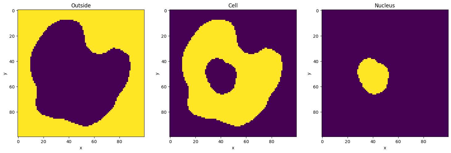
Display geometry of compartments
[10]:
fig, axs = plt.subplots(nrows=1, ncols=len(my_model.compartments), figsize=(18, 12))
for ax, compartment in zip(axs, my_model.compartments):
    ax.imshow(compartment.geometry_mask[0], interpolation="none")
    ax.set_title(f"{compartment.name}")
    ax.set_xlabel("x")
    ax.set_ylabel("y")
plt.show()
Display parameter names and values
[11]:
my_reac = my_model.compartments["Nucleus"].reactions["A to B conversion"]
print(my_reac)
for param in my_reac.parameters:
    print(param)
<sme.Reaction>
  - name: 'A to B conversion'

<sme.ReactionParameter>
  - name: 'k1'
  - value: '0.3'
Editing model contents
Parameter values and object names can be changed by assigning new values to them
Names
[12]:
print(f"Model name: {my_model.name}")
Model name: Very Simple Model
[13]:
my_model.name = "New model name!"
print(f"Model name: {my_model.name}")
Model name: New model name!
Model Parameters
[14]:
param = my_model.parameters[0]
print(f"{param.name} = {param.value}")
param = 1
[15]:
param.value = "2.5"
print(f"{param.name} = {param.value}")
param = 2.5
Reaction Parameters
[16]:
k1 = my_model.compartments["Nucleus"].reactions["A to B conversion"].parameters["k1"]
print(f"{k1.name} = {k1.value}")
k1 = 0.3
[17]:
k1.value = 0.72
print(f"{k1.name} = {k1.value}")
k1 = 0.72
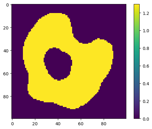
Species Initial Concentrations
can be Uniform (
float), Analytic (str) or Image (np.ndarray)
[18]:
species = my_model.compartments["Cell"].species[0]
print(
    f"Species '{species.name}' has initial concentration of type '{species.concentration_type}', value '{species.uniform_concentration}'"
)
species.uniform_concentration = 1.3
print(
    f"Species '{species.name}' has initial concentration of type '{species.concentration_type}', value '{species.uniform_concentration}'"
)
plt.imshow(species.concentration_image[0])
plt.colorbar()
plt.show()
Species 'A_cell' has initial concentration of type 'SpatialDataType.Uniform', value '0.0'
Species 'A_cell' has initial concentration of type 'SpatialDataType.Uniform', value '1.3'
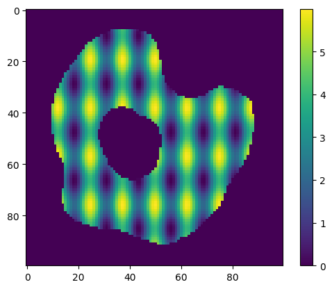
[19]:
species.analytic_concentration = "3 + 2*cos(x/2)+sin(y/3)"
print(
    f"Species '{species.name}' has initial concentration of type '{species.concentration_type}', expression '{species.analytic_concentration}'"
)
plt.imshow(species.concentration_image[0])
plt.colorbar()
plt.show()
Species 'A_cell' has initial concentration of type 'SpatialDataType.Analytic', expression '3 + 2 * cos(x / 2) + sin(y / 3)'
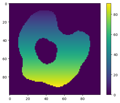
[20]:
# generate concentration image with concentration = x + y
new_concentration_image = np.zeros(species.concentration_image.shape)
for index, _ in np.ndenumerate(new_concentration_image):
    new_concentration_image[index] = index[0] + index[1]

species.concentration_image = new_concentration_image
print(
    f"Species '{species.name}' has initial concentration of type '{species.concentration_type}'"
)
plt.imshow(species.concentration_image[0])
plt.colorbar()
plt.show()
Species 'A_cell' has initial concentration of type 'SpatialDataType.Image'
Exporting a model
to save the model, including any simulation results:
model.export_sme_file('model_filename.sme')to export the model as an SBML file (no simulation results):
model.export_sbml_file('model_filename.xml')
[21]:
my_model.export_sme_file("model.sme")
[ ]: