Interactive online version

Simulating

Open an example model

!pip install -q sme
import sme
from matplotlib import pyplot as plt
import numpy as np

my_model = sme.open_example_model()

Running a simulation

• models can be simulated by specifying the total simulation time, and the interval between images

• the simulation returns a list of SimulationResult objects, each of which contains

  • time_point: the time point

  • concentration_image: an image of the species concentrations at this time point

  • species_concentration: a dict of the concentrations for each species at this time point

sim_results = my_model.simulate(simulation_time=250.0, image_interval=50.0)
print(sim_results[0])
print(sim_results[0].species_concentration.keys())

<sme.SimulationResult>
  - timepoint: 0
  - number of species: 5

dict_keys(['B_out', 'A_cell', 'B_cell', 'A_nucl', 'B_nucl'])

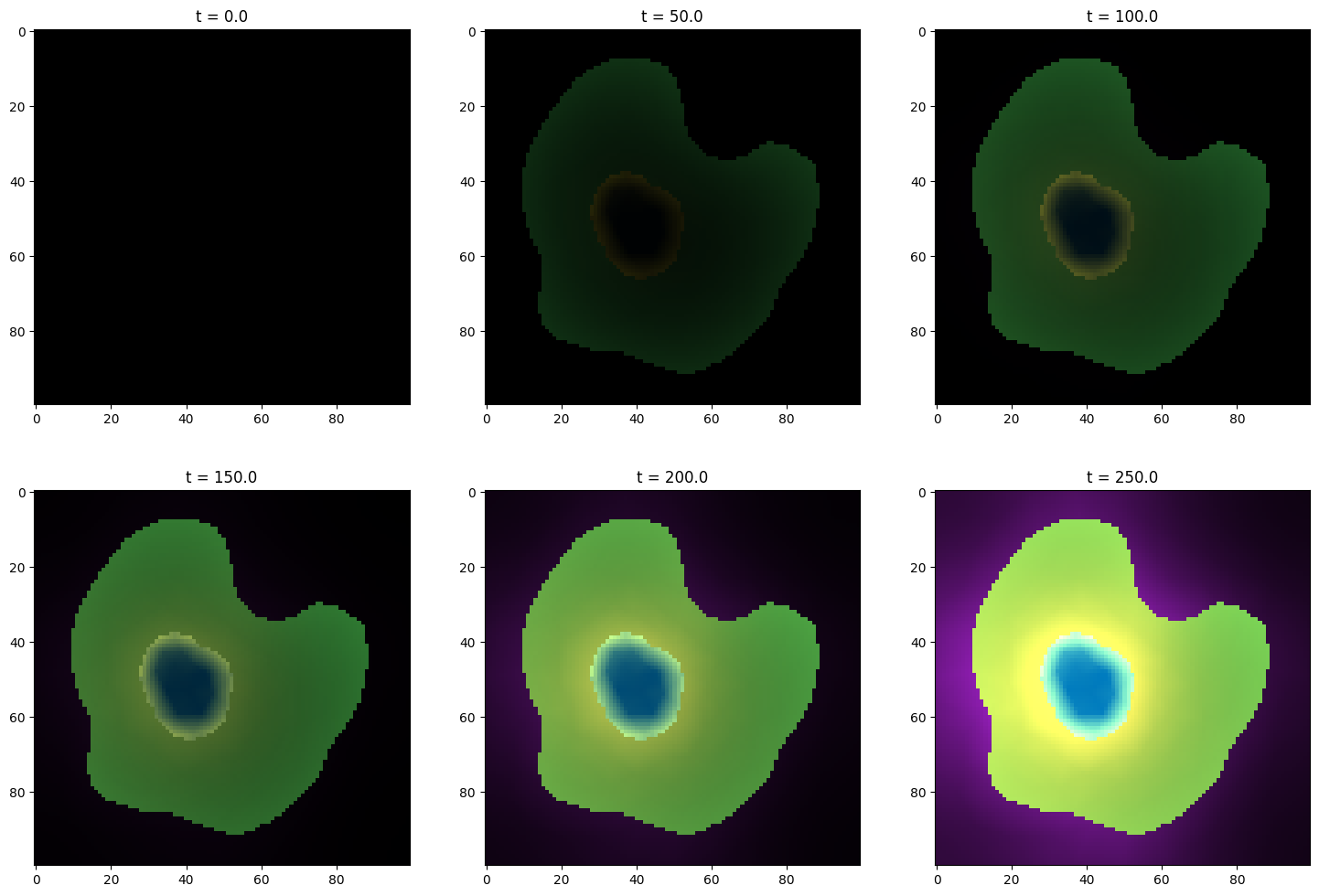
Display images from simulation results

fig, axs = plt.subplots(nrows=2, ncols=len(sim_results) // 2, figsize=(18, 12))
for ax, res in zip(fig.axes, sim_results):
    ax.imshow(res.concentration_image)
    ax.set_title(f"t = {res.time_point}")
plt.show()

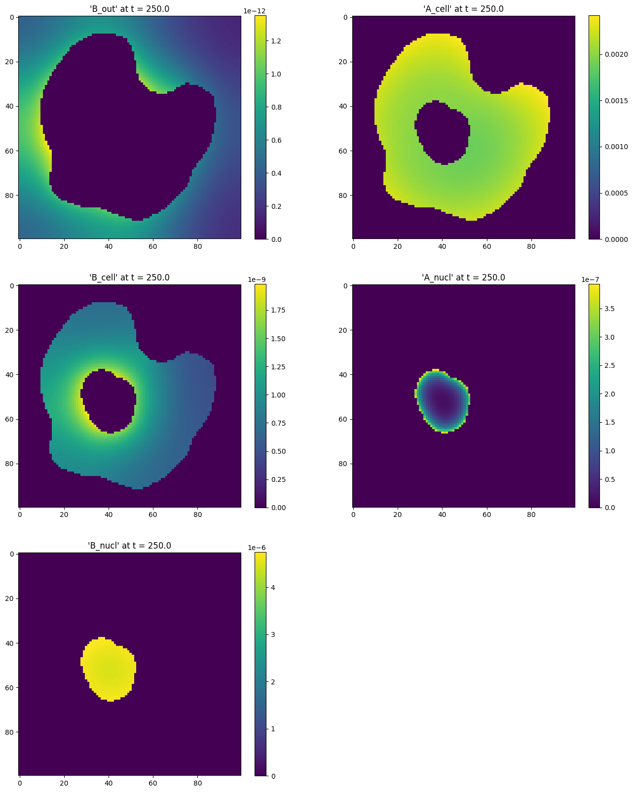
Plot concentrations from simulation results

result = sim_results[5]
fig, axs = plt.subplots(nrows=3, ncols=2, figsize=(16, 20))
fig.delaxes(axs[2, 1])
for ax, (species, concentration) in zip(fig.axes, result.species_concentration.items()):
    im = ax.imshow(concentration)
    ax.set_title(f"'{species}' at t = {result.time_point}")
    fig.colorbar(im, ax=ax)
plt.show()

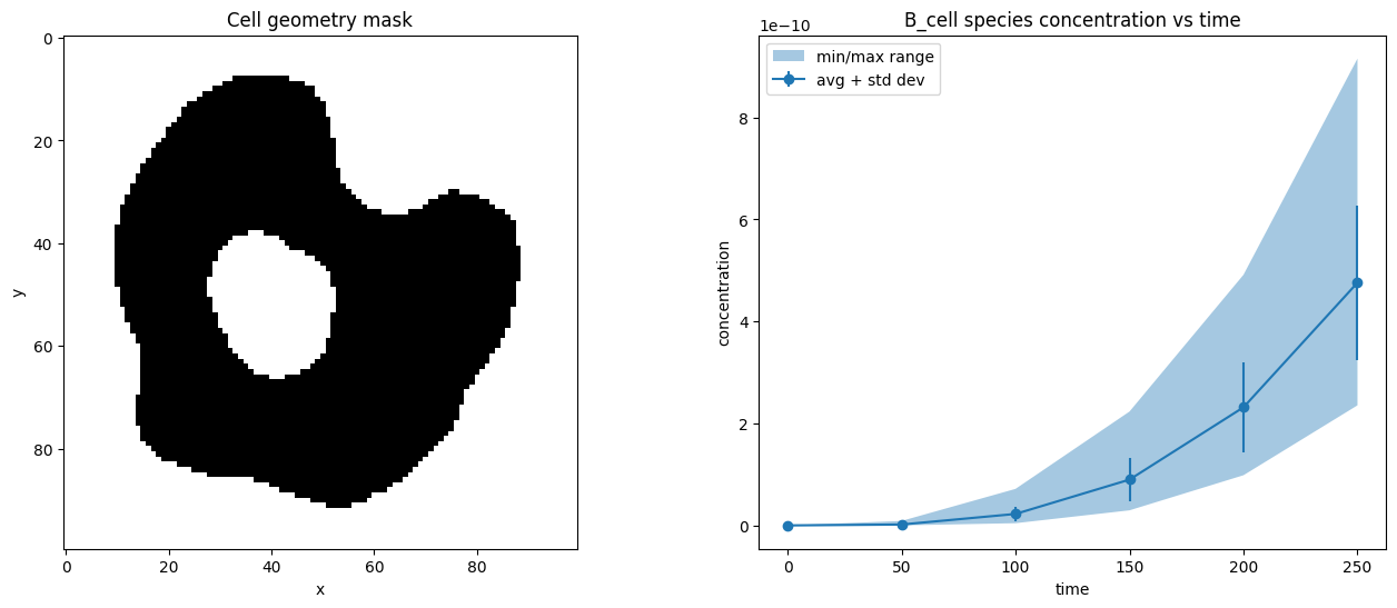
Plot average/min/max species concentrations

To get the average (or minimum/maxiumum/etc) concentration of a species in a compartment, we first use the compartment geometry_mask to only include the pixels that lie inside the compartment.

fig, (ax0, ax1) = plt.subplots(nrows=1, ncols=2, figsize=(16, 6))

# get mask of compartment pixels
mask = my_model.compartments["Cell"].geometry_mask
ax0.imshow(mask, interpolation="none", cmap="Greys")
ax0.set_title("Cell geometry mask")
ax0.set_xlabel("x")
ax0.set_ylabel("y")

# apply mask to results to get a flat array of all concentrations
# inside the compartment at each time point
times = [r.time_point for r in sim_results]
concs = [r.species_concentration["B_cell"][mask].flatten() for r in sim_results]

# calculate avg, min, max and plot
avg_conc = [np.mean(x) for x in concs]
std_conc = [np.std(x) for x in concs]
min_conc = [np.min(x) for x in concs]
max_conc = [np.max(x) for x in concs]
ax1.set_title("B_cell species concentration vs time")
ax1.set_xlabel("time")
ax1.set_ylabel("concentration")
ax1.errorbar(times, avg_conc, std_conc, label="avg + std dev", marker="o")
ax1.fill_between(times, min_conc, max_conc, label="min/max range", alpha=0.4)
ax1.legend()

plt.show()

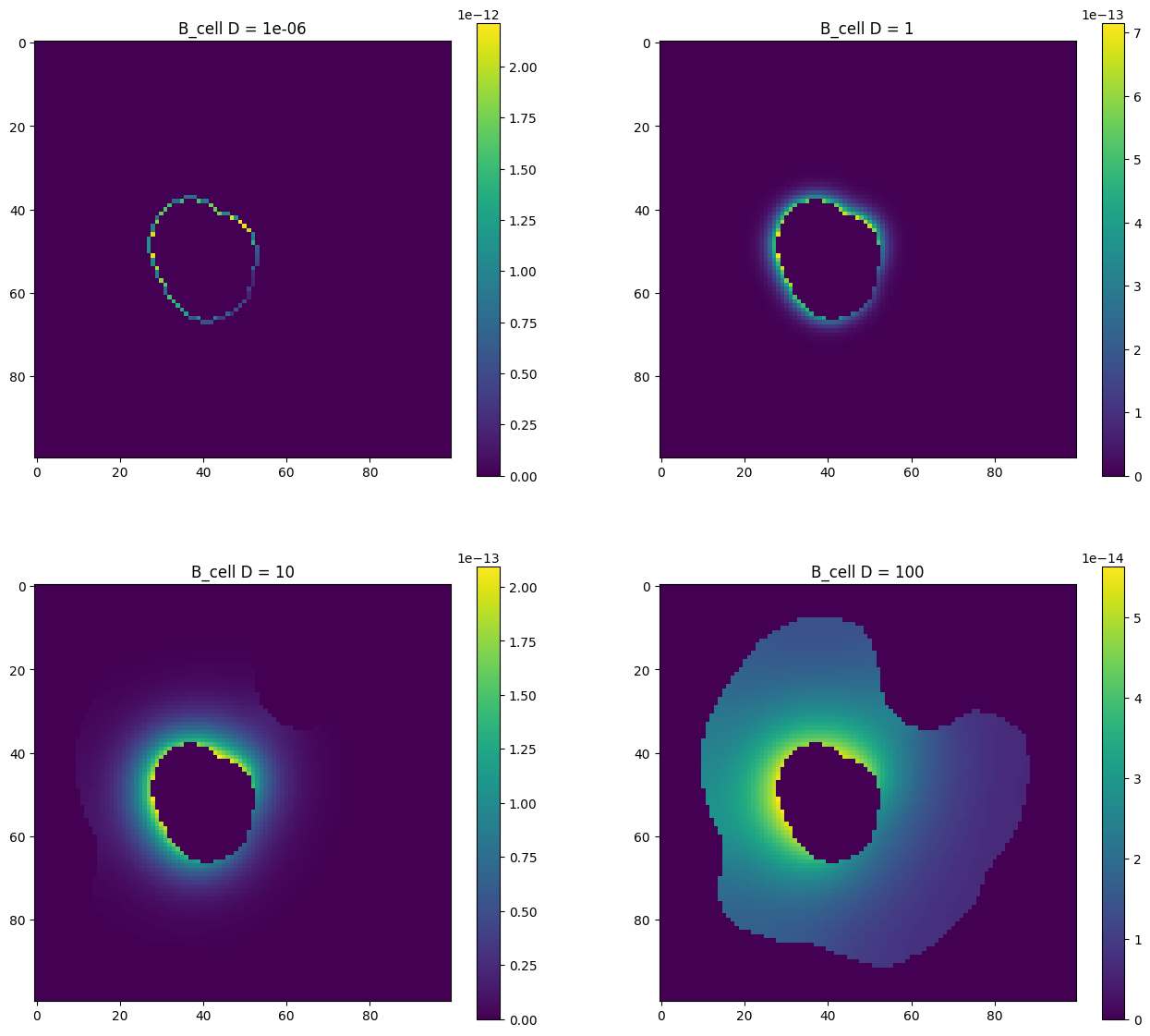
Diffusion constant example

Here we repeat a simulation four times, each time with a different value for the diffusion constant of species B_cell, and plot the resulting concentration of this species at t=15.

diffconsts = [1e-6, 1, 10, 100]
fig, axs = plt.subplots(nrows=2, ncols=2, figsize=(16, 14))
for ax, diffconst in zip(fig.axes, diffconsts):
    m = sme.open_example_model()
    m.compartments["Cell"].species["B_cell"].diffusion_constant = diffconst
    results = m.simulate(simulation_time=15.0, image_interval=15.0)
    im = ax.imshow(results[1].species_concentration["B_cell"])
    ax.set_title(f"B_cell D = {diffconst}")
    fig.colorbar(im, ax=ax)
plt.show()